Next: 6 Photoionization model Up: Observations and three-dimensional ionization Previous: 4 Plasma diagnostics
We derived ionic abundances for SuWt 2 using the observed CELs and
the optical recombination lines (ORLs).
We determined abundances for ionic species of N, O, Ne, S and Ar from CELs.
In our determination, we adopted the mean ![]() ([O III]) and the upper limit of
([O III]) and the upper limit of ![]() ([S II]) obtained from our empirical analysis in Table 4.
Solving the equilibrium equations, using EQUIB, yields level populations and line sensitivities for given
([S II]) obtained from our empirical analysis in Table 4.
Solving the equilibrium equations, using EQUIB, yields level populations and line sensitivities for given ![]() and
and ![]() . Once the level population are solved, the ionic abundances, X
. Once the level population are solved, the ionic abundances, X![]() /H
/H![]() , can be derived from the observed line intensities of CELs.
We determined ionic abundances for He from the measured intensities of ORLs using the effective recombination coefficients from
Storey & Hummer (1995) and Smits (1996).
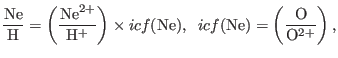
We derived the total abundances from deduced ionic abundances using the ionization correction factor (
, can be derived from the observed line intensities of CELs.
We determined ionic abundances for He from the measured intensities of ORLs using the effective recombination coefficients from
Storey & Hummer (1995) and Smits (1996).
We derived the total abundances from deduced ionic abundances using the ionization correction factor (![]() ) formulae given by Kingsburgh & Barlow (1994):
) formulae given by Kingsburgh & Barlow (1994):
| Nebula abundances | Stellar parameters | |||
| Model 1 | He/H | 0.090 |
|
140 |
| C/H | 4.00( |
|
700 | |
| N/H | 2.44( |
|||
| O/H | 2.60( |
H:He | 8:2 | |
| Ne/H | 1.11( |
|
|
|
| S/H | 1.57( |
|
3.0 | |
| Ar/H | 1.35( |
|
7500 | |
| Model 2 | He/H | 0.090 |
|
160 |
| C/H | 4.00( |
|
600 | |
| N/H | 2.31( |
|||
| O/H | 2.83( |
He:C:N:O | 33:50:2:15 | |
| Ne/H | 1.11( |
|
||
| S/H | 1.57( |
|
3.0 | |
| Ar/H | 1.35( |
|
||
| Nebula physical parameters | ||||
|
|
0.21 | 2300 | ||
|
|
100cm |
|
||
|
|
50cm |
|
||
We derived the ionic and total nitrogen abundances from ![]() N II
N II![]()
![]() 6548 and
6548 and ![]() 6584 CELs. For
optical spectra, it is possible to derive only N
6584 CELs. For
optical spectra, it is possible to derive only N![]() , which mostly
comprises only a small fraction (
, which mostly
comprises only a small fraction (![]() -30%) of the total nitrogen
abundance. Therefore, the oxygen abundances were used to correct the
nitrogen abundances for unseen ionization stages of N
-30%) of the total nitrogen
abundance. Therefore, the oxygen abundances were used to correct the
nitrogen abundances for unseen ionization stages of N![]() and
N
and
N![]() . Similarly, the total Ne/H abundance was corrected for undetermined Ne
. Similarly, the total Ne/H abundance was corrected for undetermined Ne![]() by using the oxygen abundances. The
by using the oxygen abundances. The
![]() 6716,6731 lines usually detectable in PN are preferred to be used for the determination of S
6716,6731 lines usually detectable in PN are preferred to be used for the determination of S![]() /H
/H![]() , since the
, since the
![]() 4069,4076 lines are usually enhanced by recombination contribution,
and also blended with O II lines. We notice that the
4069,4076 lines are usually enhanced by recombination contribution,
and also blended with O II lines. We notice that the
![]() 6716,6731
doublet is affected by shock excitation of the ISM interaction, so the S
6716,6731
doublet is affected by shock excitation of the ISM interaction, so the S![]() /H
/H![]() ionic abundance must be lower.
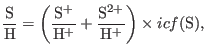
When the observed S
ionic abundance must be lower.
When the observed S![]() is not appropriately determined, it is possible to use the expression given by Kingsburgh & Barlow (1994) in the calculation, i.e.
is not appropriately determined, it is possible to use the expression given by Kingsburgh & Barlow (1994) in the calculation, i.e.
![]() .
.
| Line |
|
|
|
| 3726 |
309.42 | 335.53 | |
| 3729 |
* | 408.89 | 443.82 |
| 3869 |
204.57:: | 208.88 | 199.96 |
| 4069 |
1.71:: | 1.15 | 1.25 |
| 4076 |
- | 0.40 | 0.43 |
| 4102 H |
22.15: | 26.11 | 26.10 |
| 4267 C II | - | 0.27 | 0.26 |
| 4340 H |
38.18: | 47.12 | 47.10 |
| 4363 |
6.15 | 10.13 | 9.55 |
| 4686 He II | 43.76 | 42.50 | 41.38 |
| 4740 |
1.94 | 2.27 | 2.10 |
| 4861 H |
100.00 | 100.00 | 100.0 |
| 4959 |
216.72 | 243.20 | 238.65 |
| 5007 |
724.02 | 725.70 | 712.13 |
| 5412 He II | 5.68 | 3.22 | 3.14 |
| 5755 |
7.64 | 21.99 | 21.17 |
| 5876 He I | 6.54 | 8.01 | 8.30 |
| 6548 |
321.94 | 335.22 | 334.67 |
| 6563 H |
286.00 | 281.83 | 282.20 |
| 6584 |
1021.68 | 1023.78 | 1022.09 |
| 6678 He I | 1.63 | 2.25 | 2.33 |
| 6716 |
70.36 | 9.17 | 10.21 |
| 6731 |
46.47 | 6.94 | 7.72 |
| 7065 He I | 1.12 | 1.59 | 1.63 |
| 7136 |
15.51 | 15.90 | 15.94 |
| 7320 |
5.93 | 10.60 | 11.17 |
| 7330 |
3.37 | 8.64 | 9.11 |
| 7751 |
9.60 | 3.81 | 3.82 |
| 9069 |
5.65 | 5.79 | 5.58 |
| 1.95 | 2.13 | 2.12 |
![\includegraphics[width=1.75in]{figures/fig6_AbNIICEL.eps}](img291.png) ![\includegraphics[width=1.75in]{figures/fig6_AbOIIICEL.eps}](img292.png) ![\includegraphics[width=1.75in]{figures/fig6_AbSIICEL.eps}](img293.png) |
The total abundances of He, N, O, Ne, S, and Ar derived from our empirical analysis for selected regions of the nebula are given in Table 5.
From Table 5
we see that SuWt 2 is a nitrogen-rich PN, which may be evolved from a massive progenitor (![]() ). However, the nebula's age (23400-26300 yr) cannot be associated with faster evolutionary time-scale of a massive progenitor, since the evolutionary time-scale of
). However, the nebula's age (23400-26300 yr) cannot be associated with faster evolutionary time-scale of a massive progenitor, since the evolutionary time-scale of
![]() calculated by Blöcker (1995) implies a short time-scale (less than 8000yr) for the effective temperatures and the stellar luminosity (see Table2)
that are required to ionize the surrounding nebula.
So, another mixing mechanism occurred during AGB nucleosynthesis, which further increased the Nitrogen abundances in SuWt 2.
Mass transfer to the two A-type companions may explain this typical abundance pattern.
calculated by Blöcker (1995) implies a short time-scale (less than 8000yr) for the effective temperatures and the stellar luminosity (see Table2)
that are required to ionize the surrounding nebula.
So, another mixing mechanism occurred during AGB nucleosynthesis, which further increased the Nitrogen abundances in SuWt 2.
Mass transfer to the two A-type companions may explain this typical abundance pattern.
Fig.7 shows the spatial distribution of ionic abundance ratio N![]() /H
/H![]() , O
, O![]() /H
/H![]() and S
and S![]() /H
/H![]() derived for given
derived for given
![]() K and
K and
![]() cm
cm![]() . We notice that O
. We notice that O![]() /H
/H![]() ionic abundance is very high in the inside shell; through the assumption of homogeneous electron temperature and density is not correct. The values in Table5 are obtained using the mean
ionic abundance is very high in the inside shell; through the assumption of homogeneous electron temperature and density is not correct. The values in Table5 are obtained using the mean ![]() ([O III]) and
([O III]) and ![]() ([S II]) listed in Table 4. We notice
that O
([S II]) listed in Table 4. We notice
that O![]() /O
/O![]() for the interior and O
for the interior and O![]() /O
/O![]() for the ring.
Similarly, He
for the ring.
Similarly, He![]() /He
/He![]() for the interior and He
for the interior and He![]() /He
/He![]() for the ring. This means that there are many more ionizing photons in the inner region than in the outer region, which hints at the presence of a hot ionizing source in the centre of the nebula.
for the ring. This means that there are many more ionizing photons in the inner region than in the outer region, which hints at the presence of a hot ionizing source in the centre of the nebula.


![$\displaystyle \footnotesize {{icf}}({\rm S})= \left[1-\left(1-\frac{{\rm O}^{+}}{{\rm O}}\right)^{3}\right]^{-1/3},$](img259.png)
